Convection-diffusion in single-phase flow in porous media
Fingering and channeling
For single-phase flow in porous media, the mobility of a the fluid is defined by $k/\mu$, i.e., permeability (which is a property of the porous medium) over viscosity (a property of the fluid). Fingering and channeling terms refer to a phenomenon, where a fluid moves faster than the fluid in its surrounding zones due to the higher mobility in that particular zone of the porous medium. If this higher mobility is due to a higher permeability of the zone, the phenomenon is called channeling, and if the higher mobility is due to a lower viscosity, it is called fingering. Unlike channeling, viscous fingering can happen in an ideal homogeneous field. To initialize the fingers in numerical simulations, we often perturb slightly the permeability field. The other day, my supervisor ask me to investigate if this perturbation can indeed cause channeling in my simulations. One way to make a distinction between these two phenomenon is a tracer test, in which we inject a single phase fluid with a known concentration of a tracer into a heterogeneous field, saturated with the same fluid with zero concentration of the tracer. The concentration of the tracer does not change the properties of the fluid. We gradually increase the heterogeneity and observe its effect on the propagation of the concentration profile. We want to be certain that the small perturbation that we use to initialize the fingers does not lead to channeling phenomenon.
Single-phase flow in porous media
Flow of a Newtonian fluid in porous media is governed by the Darcy's law, which is basically an empirical relation between the permeability of the porous medium ($k$), the viscosity of the fluid ($\mu$), the superficial velocity of the fluid ($u$), and the pressure gradient ($\nabla p$): $$\mathbf{u}=-\frac{k}{\mu}\nabla p$$
For the flow of an incompressible single-phase fluid, the continuity equation reads $$\nabla.\mathbf{u}=\nabla.(-\frac{k}{\mu}\nabla p)=0$$
Finally, the convection-diffusion equation in porous media is defined by $$\varphi \frac{\partial c}{\partial t}+\nabla.(\mathbf{u}c-\varphi D \nabla c) =0,$$ where $\varphi$ is the porosity, $c$ is the concentration of the tracer or solute in mole per unit volume of the fluid, and $D$ is the diffusion coefficient.
The initial condition is zero concentration, and the boundaries are Dirichlet on the left border, and Neumann on the right border.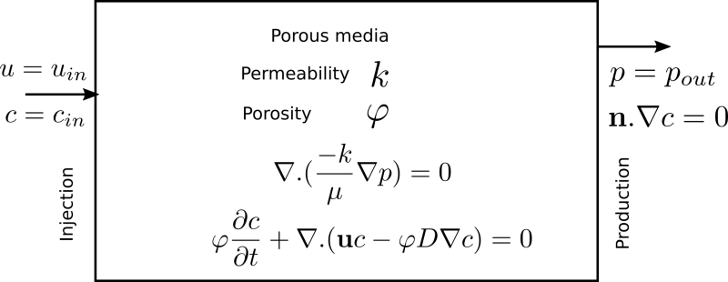
Let me implement it here.
using JFVM, PyPlot, JFVMvis
Find the pressure profile
First, we solve the diffusion equation to find the pressure profile. Then, we will use the pressure gradient to find the velocity vector. The velocity vector will be part of the convection-diffusion equation.
Nx=50
Ny=50
Lx=1.0 # [m]
Ly=1.0 # [m]
# physical values
D_val=1.0e-9 # [m^2/s]
mu_val=1e-3 # [Pa.s]
poros=0.2
perm_val=1.0e-12 # [m^2]
clx=0.05
cly=0.05
V_dp=0.02
perm= permfieldlogrndg(Nx,Ny,perm_val,V_dp,clx,cly)
# physical system
u_inj=1.0/(3600*24) # [m/s]
c_init=0.0
c_inj=1.0
p_out=100e5 # [Pa]
# create mesh and assign values to the domain
m= createMesh2D(Nx, Ny, Lx, Ly)
k=createCellVariable(m, perm)
phi=createCellVariable(m,poros)
D=createCellVariable(m, D_val)
# Define the boundaries
BCp = createBC(m) # Neumann BC for pressure
BCc = createBC(m) # Neumann BC for concentration
# change the right boandary to constant pressure (Dirichlet)
BCp.right.a .= 0.0
BCp.right.b .=1.0
BCp.right.c .=p_out
# left boundary
BCp.left.a .= -perm_val/mu_val
BCp.left.c .= u_inj
# change the left boundary to constant concentration (Dirichlet)
BCc.left.a .= 0.0
BCc.left.b .= 1.0
BCc.left.c .= 1.0
labda_face=harmonicMean(k/mu_val)
Mdiffp=diffusionTerm(labda_face)
Mbcp, RHSp = boundaryConditionTerm(BCp)
Mp= Mdiffp+Mbcp
p_val=solveLinearPDE(m, Mp, RHSp)
figure(figsize=(5,4))
visualizeCells(p_val)
title("Pressure profile [Pa]")
colorbar();

Solve the convection-diffusion equation
Now we have the velocity profile, that we will use to define and solve the convection-diffusion equation.
# estimate a practical time step
n_loop=50
dt=Lx/u_inj/(5*100) # [s]
# find the velocity vector
u=-labda_face*gradientTerm(p_val) # [m/s]
# find the matrices of coefficients
D_face=harmonicMean(phi*D)
Mdiffc=diffusionTerm(D_face)
Mconvc=convectionUpwindTerm(u)
Mbcc, RHSbcc = boundaryConditionTerm(BCc)
# initialize
c_old = createCellVariable(m, c_init, BCc)
c_val = copyCell(c_old)
# start the loop
for i=1:n_loop
    (Mtransc, RHStransc) = transientTerm(c_old, dt, phi)
    Mc=-Mdiffc+Mconvc+Mbcc+Mtransc
    RHSc=RHSbcc+RHStransc
    c_val=solveLinearPDE(m, Mc, RHSc)
    c_old=copyCell(c_val)
end
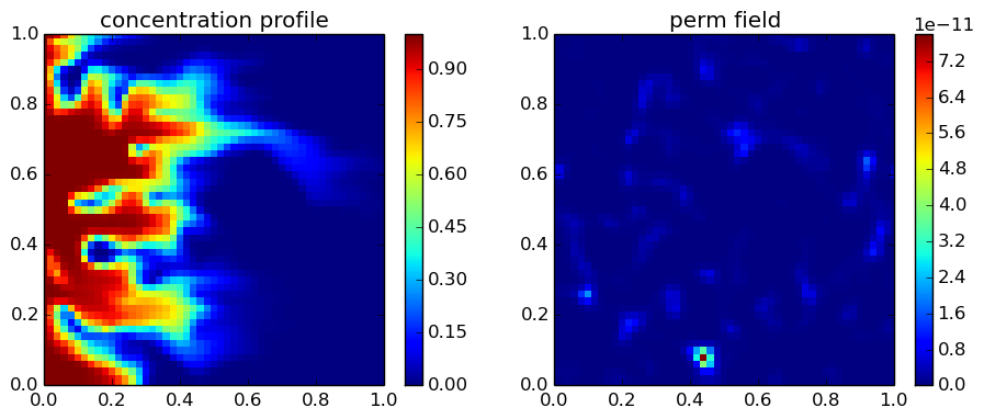
figure(figsize=(11,4))
subplot(1,2,1)
visualizeCells(c_old)
title("concentration profile")
colorbar();
subplot(1,2,2)
visualizeCells(k)
colorbar()
title("perm field");

Conclusion
By changing the Dykstra-Parsons coefficient to a higher value, we can observe channeling phenomenon in porous media by looking at the concentration profile. A small value of Dykstra-Parsons, around 0.01, which makes a +/- 3% perturbation in the permeability field does not lead to a channeling phenomenon, and is enough to initialize the fingers. Beautiful figures can be made by assigning a value of 0.7 or 0.8 to the Dyktra-Parsons coefficient (see below)!