Conduction and diffusion: a brief tutorial
Important Update: the codes in this post will not work with the new version of FVTool. Download the old version of FVTool here.
Warning
This post is not edited. You may find horrible English mistakes.
Diffusion/conduction equation; mass and heat transfer
As a chemical engineer mass transfer is my favorite topic, which is sort of strange given the fact that heat transfer is way easier to feel and understand. It has to be due to the very busy schedule of my heat transfer Professor, who was involved in a project at the time and did not spend enough time on getting ready for his teaching duties, unlike my mass transfer Professor. Back to business...
Temperature gradient is the driving force behind the conductive heat transfer, and the gradient of chemical potential is the driving force behind the diffusive mass transfer. At low concentrations, the gradient of the chemical potential can be replaced by the concentration gradient. Here I'm going to show you how to solve a conservation equation when the only flux term is the diffusive heat or conductive mass (doesn't sound as funny as I expected). The equation reads
$$ \nabla . (-\lambda \nabla \phi)=q, $$
where for mass transfer, $\lambda$ denotes the diffusivity (m^2/s) and $\phi$ denotes the concentration (mol/m^3), and q is a mass source term (mol/(m^3.s)) and for heat transfer, $\lambda$ denotes the conductivity (J/(m.K.s)) and $\phi$ denotes the temperature (K), and q is a heat source term (J/(m^3.s)). There are other physical phenomena that can be described by the above relation, e.g., Poisson equation or flow in porous media, in which $\lambda$ denotes the total mobility (permeability divided by the viscosity for single phase flow), and $\phi$ denotes pressure.
Boundary conditions
I think Dirichlet (constant value) and Neumann (constant flux) boundary conditions are quite clear in terms of their physical meaning. However, there are two important situations that lead to a Robin boundary condition. In heat transfer, when a boundary is gaining/losing heat to a medium with a constant temperature of $$ T_{\infty} $$ by convection mechanism with a heat transfer coefficient h (J/(m^2.K.s)), the energy balance equation at the boundary reads
$$ -\lambda (\mathbf{n}.\nabla T) = h(T-T_{\infty}), $$
which can be rearranged to the following form that can be formulated in the FVMtool:
$$\frac{\lambda}{h} (\mathbf{n}.\nabla T) + T = T_{\infty}$$
For the mass transfer, if mass is produced or consumed at a boundary by a first order reaction rate, the equation reads
$$ -\lambda (\mathbf{n}.\nabla c) = k_0 c, $$
where $k_0$ is the rate constant of the reaction that happens on the boundary. For a chapter of my thesis, I encountered this sort of boundaries and it was the main reason that I rewrote the implementation of boundary condition from scratch. I will talk about the implementation of the boundary conditions later in a separate post.
A (sort of) real problem
Fins are used to increase the heat transfer area and thus the rate of heat transfer. Here we are going to model a fin in 2D. The base of the rectangular fin is attached to a surface with a constant temperature of 100 degree Celsius. The fin is made of Aluminum, with a thermal conductivity of 237 W/(m.K), with a thickness of 0.1 cm and a length of 10 cm. The fin is exposed to a air at a constant temperature of 25 degree Celsius, and the heat transfer coefficient is 10 W/(m^2.K). This number may be off so you can estimate it using one of these correlations.
Let us jump into our Matlab FVTool, and solve this problem numerically using the finite volume method.
Solution procedure
First, we start by defining the domain and creating the mesh structure:
clc; clear; % clean the command prompt, clean the memory
L = 0.1; % 10 cm length
W = 0.01; % 1 cm thickness
Nx = 50; % number of cell in x direction
Ny = 20; % number of cells in the y direction
m = createMesh2D(Nx, Ny, L, W); % creates a 2D Cartesian grid
Now, we define the the transfer coefficients. We assume that the thermal conductivity is constant on the whole domain. However, we need to assign this constant value to each individual cell. This is done by the function createCellVariable. After creating this thermal conductivity field, we have to calculate the average values on the interface between cells or the faces. Again, in this special case, the average values are equal to a constant. But in other cases when the conductivity varies with space, the averaging becomes more important. Three averaging techniques are available in the FVTool, viz. arithmetic, geometric, and harmonic. The output of these averaging functions is always a face variable. Let's see that in action:
T_inf = 25+273.15; % [K] ambient temperature
T_base = 100+273.15; % [K] temperature at the base of the fin
k_val = 237; % W/(m.K) thermal conductivity
h_val = 10; % W/(m^2.K) heat transfer coefficient
k = createCellVariable(m, k_val); % assign thermal cond. value to all cells
k_face = geometricMean(m, k); % geometric average of the thermal conductivity values on the cell faces
Now, we can define the boundary conditions. Here, we have one Dirichlet (constant temperature) and three Robin boundaries. The general boundary condition is defined as
$$ a (\mathbf{n}.\nabla \phi)+b\phi = c. $$
a, b, and c must be defined in the program. Here, we have $a=\lambda/h$, $b=1$, and $c=T_{\infty}$. Don't forget to include the sign of the normal vector for the bottom boundary. The normal vector is in the opposite direction of the y axis and therefore its sign must be included in the temperature gradient term. I will talk about it in more details later.
BC = createBC(m); % creates a BC structure for the domain m; all Neumann boundaries
BC.left.a(:)=0; BC.left.b(:)=1; BC.left.c(:)=T_base; % convert the left boundary to constant temperature
BC.right.a(:)=k_val/h_val; BC.right.b(:)=1; BC.right.c(:)=T_inf; % right boundary to Robin
BC.top.a(:)=k_val/h_val; BC.top.b(:)=1; BC.top.c(:)=T_inf; % top boundary to Robin
BC.bottom.a(:)=-k_val/h_val; BC.bottom.b(:)=1; BC.bottom.c(:)=T_inf; % bottom boundary to Robin
Now, we have a domain with fully specified transfer coefficients and defined boundary. Next and final step is to find the matrix of coefficients for the conduction term and the boundary conditions, and solve the linear system of discretized linear equations:
M_cond = diffusionTerm(m, k_face); % matrix of coefficients for the heat diffusion
[M_bc, RHS_bc] = boundaryCondition(m, BC); % matrix of coefficients and RHS vector for the boundary conditions
T = solvePDE(m, M_cond+M_bc, RHS_bc); % solve the linear system of discretized PDE
visualizeCells(m, T); % visualize the results
Little fun
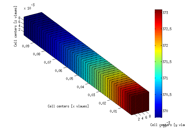
Please find the source code for this tutorial here. To have some numerical fun, try to change the problem from 2D to 3D by activating the appropriate line in the Matlab source code. You can also increase the heat transfer coefficient and see its effect on the temperature profile. In the next post, I will explain how to convert this example to a unsteady-state simulation.
This is a snapshot of the 3D result: